
A transport model is devised with two primary requirements: replicating base year situations and forecasting future year implications.
To achieve an acceptable validation performance, measures are sometimes introduced which compromise the quality of the forecasting performance of the model. Overfitting the base year can undermine the reliability of the forecasting outcomes. This article explores the impact of ‘overfitting’ through three case studies that cover the three model components: trip generation, trip distribution and mode choice.
The use of special generators to improve base year performance can compromise the model’s forecasting capability. We demonstrate an alternative model, which although not fitting the base year data as well as the alternative, does provide a better forecasting outcome.
Alternative A produces good results for the largest shopping centre A, after the adjustment factor of 2.5 is applied based on the observed traffic counts. Alternative B produces considerably worse validation results for the largest centres, but notably better outcomes for relatively smaller centres.
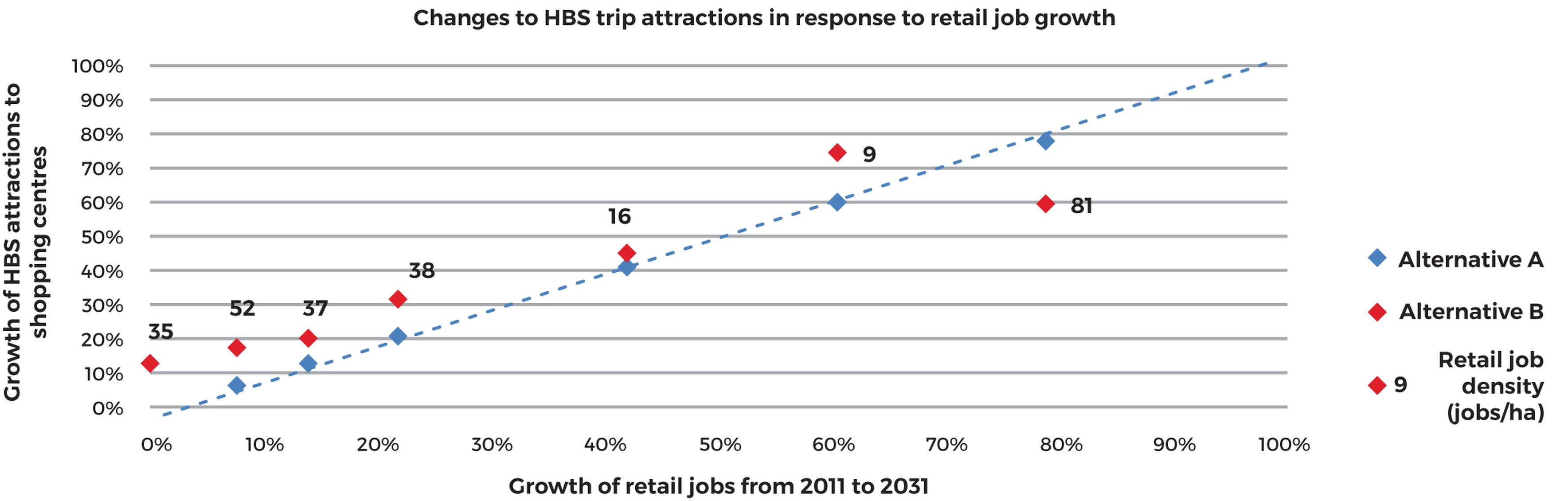
In terms of forecasting outcomes, Figure 1 illustrates the increase of HBS trip attraction to the shopping centres from 2011 to 2031, in response to the growth of retail jobs. It shows that in Alternative A, trip attractions increase in a linear fashion with growth in jobs, whilst Alternative B reflects the density effect for forecasting: trip attractions increase at a faster rate when the growth is added to a site with a relatively low job density than when growth is added to a site with an already high job density.
The trip distribution model is often estimated from Household Travel Survey (HTS) data in the gravity model form. The sample sizes of HTS data typically result in very sparse matrices, where many origin-destinations (OD) have zero observed trips. Many of the zero cells are ‘true’ zero meaning that there are no trips in reality, whilst the remaining ones are ‘false’ zero due to sampling though non-zero demand does exist in real world. Different approaches for treating the zero values are demonstrated as follows:
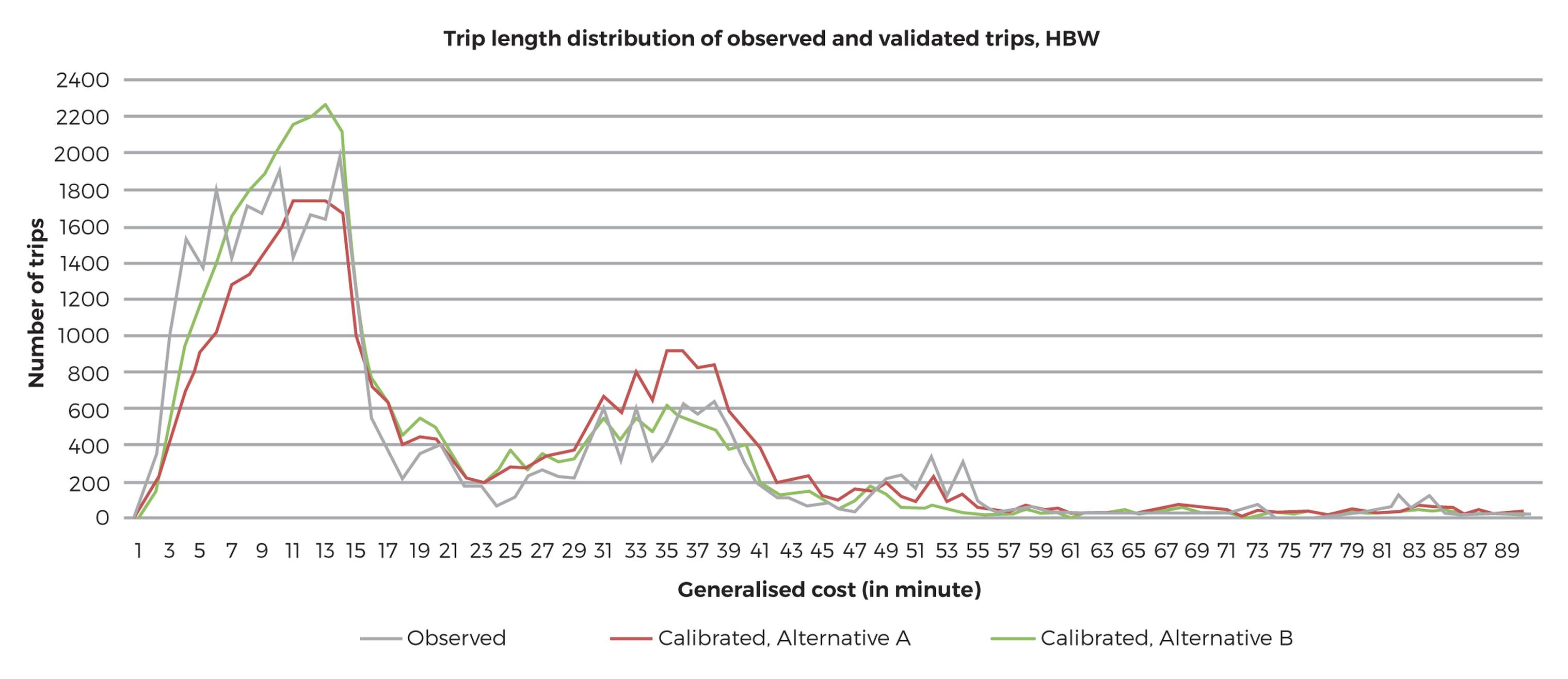
Figure 2 illustrates the trip length comparison by using observed trip productions and attractions (P&As) as inputs for applying the trip distribution formulation and producing outturn trip lengths. It shows that Alternative A produces a significantly better fit to the observed data that Alternative B. As Alternative B uses modelled P&As to calibrate the model parameters, not observed, this difference in fit is expected.
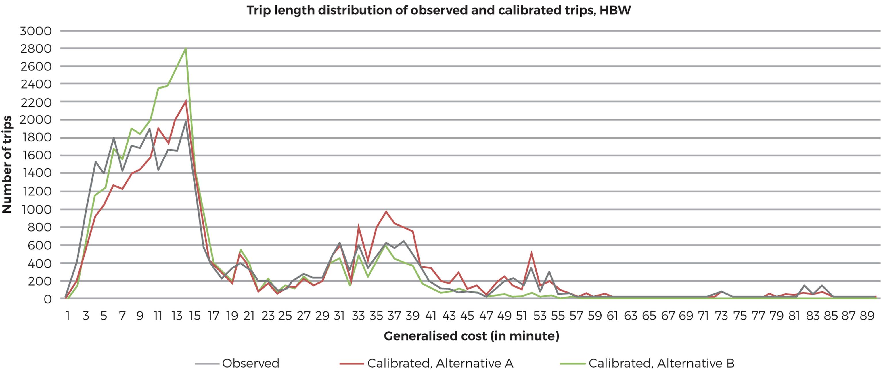
However, in actual model applications, modelled productions and attraction totals are input to the distribution model, not observed trip ends. In that case, as shown in Figure 3, Alternative A produces significantly longer average trip lengths compared with the HTS data, when the observed P&As are replaced with modelled values for producing outturn trip lengths. In contrast, Alternative B produces good fitness to the observed trip lengths.
In terms of forecasting outcome, Alternative B produces a more sensitive model response than Alternative A. The elasticity of changes in trip length in response to generalised cost increase for Home Base Shopping trips is about -0.17 for Approach A and -0.27 for Approach B in our case study.
This may mean that model development effort improving the base year might be better spent critically examining the performance of the model in forecasting together with developing a range of forecasts and sensitivity tests
In many four-step models the mode choice occurs after the trip distribution (or destination choice). This ordering is computationally convenient: trip distribution yields a set of origin-destination tables; the mode choice component then determines which modes of transport are used for each OD pair, while taking account of travel cost from the origin to destination as one of inputs. Arguably, this order also fits in a modellers’ experience of real life in so far as on many occasions travelers decide on their destinations first and then choose between transport modes.
The reverse order, implementing mode choice before destination choice, is less computationally straightforward: the destinations from production zones are unknown meaning that the generalised cost input for mode choice must be aggregated or composed at trip production level, instead of at trip (origin-destination) level. Due to the aggregation of cost inputs, the resultant base year validation outcomes tend to be less desirable than the destination choice first approach. More importantly, the sequence affects elasticities of demand to cost/disutility changes and therefore, predicted future year demand.
This case study compares the base year validation and future year sensitivity between the two different sequences for Home Based Shopping trips. The estimation of the destination and mode choice models uses a utility maximising method that is now commonly adopted in strategic level demand models, and is well described in the literature.
We found that both approaches produced reasonable base year validation outcomes in terms of the comparison between observed and modelled mode shares. However, for the isolated origin-destination movement used in the case study, the mode choice first approach produces more sensible and sensitive outcomes in response to the model input changes in either single constrained or double constrained setting.
Overfitting measures can reduce a model’s responsiveness to the changes in model inputs, undermining the reliability of forecasting outcomes. The alternative models that remove the over-fitting measures may have less desirable validation outcomes, but can produce more responsive and sensible outcomes in forecasting. Our conclusion is that recognising relative underperformance in the base year validation in exchange for more reasonable forecasting outcomes may be preferred to overfitting to observed data.
In practice, this may mean that model development effort improving the base year might be better spent testing the model’s performance in forecasting, critically examining the performance of the model in forecasting together with developing a range of forecasts and sensitivity tests, which explore the uncertainties attached to each of the input assumptions.
Yun Bu works in AECOM’s Dubai office
TransportXtra is part of Landor LINKS
![]()
© 2026 TransportXtra | Landor LINKS Ltd | All Rights Reserved
Subscriptions, Magazines & Online Access Enquires
[Frequently Asked Questions]
Email: subs.ltt@landor.co.uk | Tel: +44 (0) 20 7091 7959
Shop & Accounts Enquires
Email: accounts@landor.co.uk | Tel: +44 (0) 20 7091 7855
Advertising Sales & Recruitment Enquires
Email: daniel@landor.co.uk | Tel: +44 (0) 20 7091 7861
Events & Conference Enquires
Email: conferences@landor.co.uk | Tel: +44 (0) 20 7091 7865
Press Releases & Editorial Enquires
Email: info@transportxtra.com | Tel: +44 (0) 20 7091 7875
Privacy Policy | Terms and Conditions | Advertise
Web design london by Brainiac Media 2020