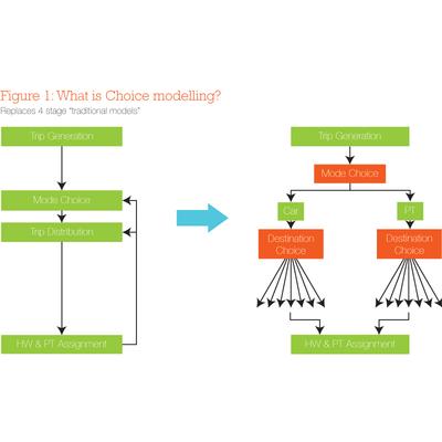
Choice modelling models people’s choices and decisions, whether they be decisions about transport, consumer purchases, activities or lifestyle. In four-stage transport modelling, the demand model can be replaced by a choice nest of mode and destination choice (as shown in Figure 1). Other choices can also be incorporated, as discussed later.
People perceive the alternatives differently and weigh things up differently, according to Random Utility Theory; people therefore make different decisions when confronted with the same set of facts. For example, of 100 car owners going to and from the same pair of places, some will choose to go by car and some by public transport, even though they all have the same set of alternatives, the same travel time alternatives with the same cost, and so on. This is because they perceive the same travel time and costs, but weigh up the options differently. In fact, their perception varies according to (something like) a normal distribution. When the mathematicians have worked through the maths this translates into the academically sound logit model (McFadden, 1974). This has been borne out by its use in practice since 1974; it is considered empirically the best model of choice that we have. Choice modelling is sometimes called discrete choice modelling or disaggregate modelling because people are considered individually.
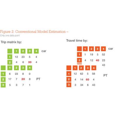
Aggregate modelling, as used in four-stage models and particularly the gravity model, deals with people in aggregate, while choice modelling deals with individuals. This is clearly illustrated by the aggregate approach to estimating (in four-stage modelling this is sometimes called calibrating) a mode choice model using, for example, travel time as the independent variable.
A trip matrix of the number of observed trips between an origin and a destination is shown in Figure 2. Between zones 2 and 3 there are 50 trips; this number can be treated as a single observation, as for aggregate modelling, or as 50 single observations in a discrete modelling approach. The power of discrete choice estimation is unlocked if we add more variables (not just the usual variables of travel time and cost) about the two modes. We can add variables about the person, for example their income (highly relevant to choice of car or public transport), about infrastructure, perhaps real-time information availability, which again could be highly relevant to their decision. So now, instead of having just a single observation, we have 50 observations to make use of. We can look for relationships, for example, between income and public transport use in our data, and design a model to capture that relationship. This means that choice models are better at explaining behaviour and forecasting traffic, ridership and revenue on new transport facilities. We get a more reliable, and potentially more accurate, forecast.
Choice modelling allows use of 'goodness-of-fit' statistics such as the ‘t’ statistic, which indicate whether a choice modelling variable is relevant to the choice, and if so how important it is. We can try lots of different variables and use those which are sufficiently important, while discarding the unimportant ones. With aggregate models, however, we remain completely in the dark.
We suggest that choice modelling can do everything that aggregate models can do, plus much more. Choice models are therefore good professional best practice, and help to meet current Government guidance (WebTag requirements). There are also many pitfalls with connecting mode and destination in aggregate, which can lead to counter-intuitive model results. Such problems arise because the benefits of the alternative choices are not properly measured in such models.
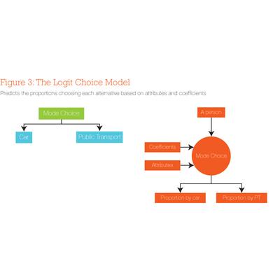
Choice modelling uses the logit model. For example, the choice of whether to go by car or public transport (see Figure 3) is given by a set of variables (called attributes) about each alternative. Each attribute is multiplied by a coefficient that essentially weights it according to the traveller's perception of it, and the utility they perceive they will get from choosing it. Travellers weigh up the utility of going by car versus going by public transport, and choose the one with the highest utility (utility can be seen as a more general form of the concept of generalised cost used in aggregate modelling).
In choice modelling, discrete choices are used to estimate the coefficients, taken from situations where people have already made the decision. This is called 'revealed preferences' because the decision-making behaviour has been revealed by actions. Choice models can also be estimated from situations where people tell you what they would choose to do in a hypothetical situation. This is called 'stated preference' data because choices have only been stated, but not carried out.
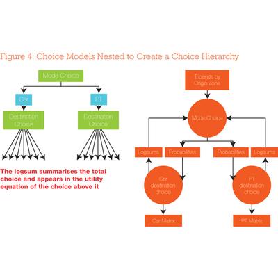
The four-stage demand model consists of both mode and destination, so choice modelling replaces these with a nest of two choices. One choice is nested underneath the other (see Figure 4). The choice models are connected through the logsum, which summarises the choice situation into one value which is passed up to the utility function of the nest above it in the hierarchy. This is used to calculate the utility of the upper nest, and hence the probability (or number of trips) of choosing each alternative. These are passed down to the next level, which calculates the probabilities, and hence the number of these trips going to each destination, for car and for public transport. This is, we suggest, the correct way of connecting mode and destination choice models.
This connection between the nests is correct with choice modelling, but can be very wrong with aggregate models. We have seen the attributes at the lower level averaged and passed up. However, modellers must always use the logsum because weighted averages can give counter-intuitive results. For example, if a new AM peak bus service is provided, or if AM peak congestion is relieved by building a bypass (and the effect is less marked in the non-AM peak), then the average all-day generalised cost reduces, resulting in changes to non-peak car traffic.
We have discussed the problems with the gravity model in a previous Modelling World session in 2012, noting that:
It can have more than one solution
The solution depends on the number of iterations you choose
The model may fail to converge, so that there may be large variations in flows between some origin-destination movements
You won’t know it is doing this unless you look for it which is not always possible when you are working rapidly through forecasts
There is no known cure (other than to use choice modelling)
The coefficient of the logsum is the sensitivity parameter, and is critical to the process. It determines which way up the nest is (whether mode is above destination or destination above mode). It also governs the sensitivity of one choice relative to the other. It is perhaps the most critical single coefficient in the whole model, since small changes in its value can lead to large changes in the forecasts. It should be estimated as part of model calibration and not guessed from other studies. There are three ways of doing this:
Use aggregate modelling methods
Consider the car destination choice as a multinomial choice, pass the logsum up to the mode choice, do the same for public transport destination choice and then estimate the mode choice model as a multinomial logit model
Do a nested logit estimation of both nest levels simultaneously
We consider the first method, using aggregate modelling methods, to be incorrect because it does not give a logsum coefficient, so it is not possible to know which way up the nest is. It does not give a ’t’ statistic, so it is not possible to know whether it is a nested logit or one big multinomial logit. It is not possible to justify forecasts at all.
The third method, in our opinion, is the correct one. The second method is not good practice due to several issues: having estimated the top level, this may change the lower level estimations so consistency may be poor.
If you must use aggregate modelling, use the logsum. Better still, use choice modelling. Convert demand models to choice models with a nested set of choices. There is plenty of software out there that can help you implement choice modelling. Available software includes our own Visual Choice, which integrates with the CUBE software from Citilabs, Visum, and with our Visual-tm software.
TransportXtra is part of Landor LINKS
![]()
© 2026 TransportXtra | Landor LINKS Ltd | All Rights Reserved
Subscriptions, Magazines & Online Access Enquires
[Frequently Asked Questions]
Email: subs.ltt@landor.co.uk | Tel: +44 (0) 20 7091 7959
Shop & Accounts Enquires
Email: accounts@landor.co.uk | Tel: +44 (0) 20 7091 7855
Advertising Sales & Recruitment Enquires
Email: daniel@landor.co.uk | Tel: +44 (0) 20 7091 7861
Events & Conference Enquires
Email: conferences@landor.co.uk | Tel: +44 (0) 20 7091 7865
Press Releases & Editorial Enquires
Email: info@transportxtra.com | Tel: +44 (0) 20 7091 7875
Privacy Policy | Terms and Conditions | Advertise
Web design london by Brainiac Media 2020